What is Data Parallelism?

Data parallelism, or just data parallel (or DP for short) is a concept from distributed training. The name is self-explanatory: given a model, we replicate the model on each of our GPUs. Each model replica, called a model instance, will run the forward and backward passes using different micro batches of data. This is done in parallel for each GPU.

Background Note On Memory Impact

Data parallelism is a technique to help us reduce the memory impact on our devices, so it's worth understanding why there's a memory impact, and it's a fair question for interviewers to ask. We discuss this more in memory components but as a quick recap, training neural networks requires saving several pieces of state in memory:

• model weights
• model gradients
• optimizer states
• activations (required for gradient calculations)

Of the above components, research show that the total memory required for the activations scales linearly with the batch size and quadratically with the sequence length. The key takeaway here is that, for large inputs (a.k.a large batch-sizes or sequences), activations become the dominant memory burden.

While activation recomputation and gradient accumulation are techniques to account for this on a single compute device, data parallelism extends the logic of gradient accumulation by parallelizing it across multiple devices.

Data Parallelism helps us to avoid the memory explosion from large batch sizes.

How It Works

By duplicating our model across N GPUs, and splitting our data (global batch) into N micro-batches, we can perform forward and backward passes in parallel on each micro-batch, on each GPU. In this manner, there's less work to do for each GPU (ignoring communication overhead, we can expect ~Nx faster training!).

Of course, if our setup has a model replica on each GPU, each receiving a different micro-batch, we'll need some form of synchronization at some point. Recall that our model goes through 3 key steps during training:

1. Forward Pass: Inputs go through model and produce outputs.
2. Backward Pass: Gradients calculated for a loss given the model weights.
3. Optimization Step: The gradients are used to update the model's parameters.

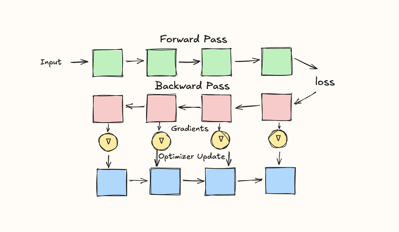
It turns out that steps 1 and 2, the forward and backward passes, respectively, can be calculated independently for each micro-batch: the forward pass just calculates the output for the given micro-batch, while the backward pass calculates the gradient of the given micro-batches loss given the weights).

However, step 3, updating the weights of our model, is more complicated. Sending a different micro-batch to each GPU means that each GPU will have different gradients. Because we want our model replicas to stay in sync, we need to sync these together before the optimizer step. We'll do this using the all-reduce operation (read our question on GPU collective operations to learn more), specifically averaging the gradients across the model instances together. (An interviewer may ask, why the average and not the sum?. The answer is simple: to ensure the result is independent of the number of gradient accumulation steps used.)

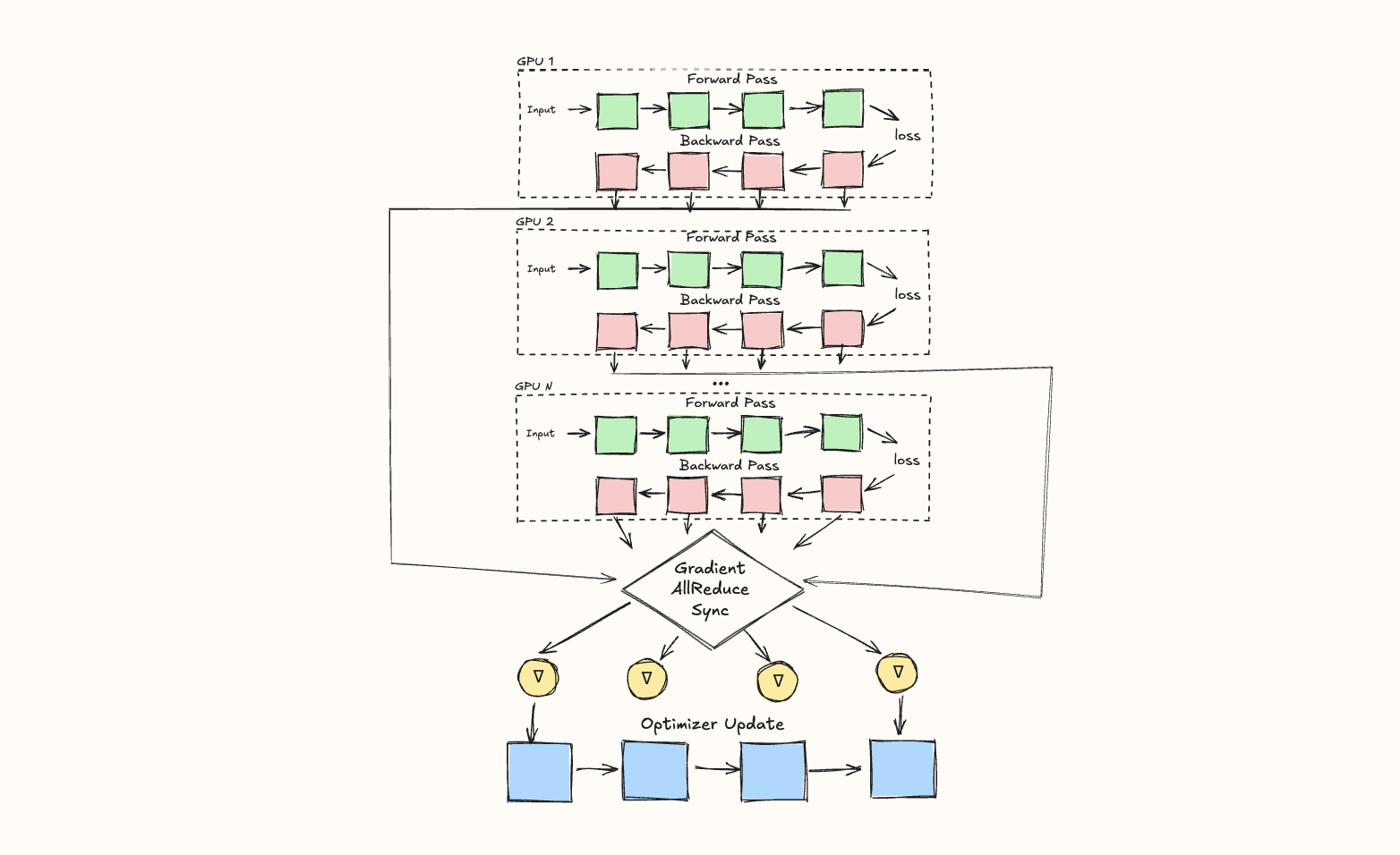
In other words, once the backward pass is finished, and we have all the gradients, we kick off an all-reduce operation over all of our DP ranks (rank just means compute device, e.g. GPU), syncing them.

Optimizing Data Parallel

Distributed training is all about keeping our GPUs idle as little as possible, so sequential steps of computation are often a sign that things can be optimized. Presenting the above information in an interview will indeed communicate that you know DP, but interviewers will likely probe you to go deeper on the subject, and talk about how you can overlap communication and computation.

There are three main ways to overlap communication and computation with data parallel:

1. Overlap gradient synchronization with backward pass: Gather and sum the gradients for a given layer before the gradients from earlier layers have been computed.

2. Bucketing Gradients: Group gradients into buckets and use a single all-reduce for all the gradients within the same bucket.

3. Combine Data Parallel and Gradient Accumulation: Use data parallel and gradient accumulation together. That is, distribute data across the GPUs, but within each GPU, use gradient accumulation as well. In this setup, you'll need to ensure you use a single all-reduce at the end, instead of one-per-backward pass.

Limitations

Data Parallelism has some core limitations:

First, the ability to increase training throughput by adding more model replicas across GPUs assumes that we can even fit a model replica (specifically, a forward pass for micro-batch size of 1) on each GPU. This isn't always true, especially for the massive models being trained today. (That said, for a small communication cost, we can use ZeRO to fit models that ordinarliy wouldn't fit on a single GPU by sharding the parmeters, gradients, and optimizers across the DP ranks.) Also, recall that earlier we mentioned the two main bottlenecks of activation memory: batch-size and sequence-length. If a model has too large a sequence-length, we may not be able to fit it either.

The second issue is scale: as the number of GPUs grows to the hundreds or thousands, the overhead communication required for the gradient all-reduce becomes prohibitively expensive.

Of course, at this point, you can start reaching for other parallelism techniques (e.g. tensor parallelism or context parallelism) to use alongside data parallelism.